
Before we proceed, checkout the news InfoCaptor recently got certified with Cloudera Impala and Hive

In this article we will analyze the NFL play by play dataset. The data consists of each play for all games from 2002 thourgh 2013. It is roughly around 600k rows and hardly qualifies as big data. The main point of this article is to illustrate the use of Cloudera Impala for Big Data anlaysis. We will also see the comparison performance against Hive.
Once connected to the Impala instance we see a list of all available schemas and tables in them.
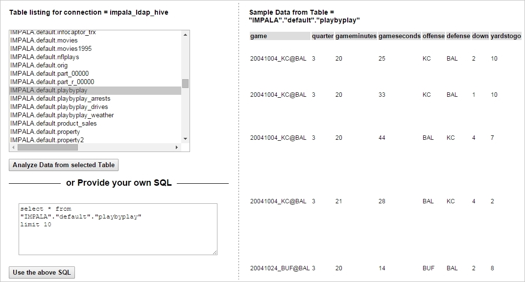
As you can see the sample data lists each play for every NFL game. With so many fields it provides lot of juice for the analysis but at the same time can be a brain jammer.
Another problem with data is that there is a mix grain, i.e Data points that are at the Game level repeat for each play.
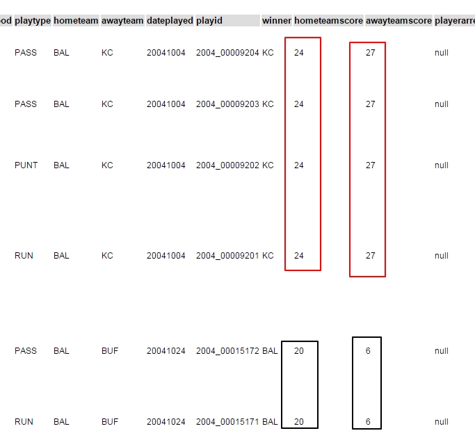
As you see the awayteam score and the hometeam score repeats for each play of the game. So we cannot simply sum the scores and group by the game id.
It would be nice if there was a flag indicating the first row of each game and then we can just filter based on that.
Analyzing the data further, it seems after applying the following filters we can exactly fetch the first row of each game.
If the playttype is kickoff, quarter is 1st, gameminutes and gameseconds both equal to zero then this combination gives us exactly the top row for each game. We don’t need so many fields for our analysis so we will create a custom SQL on top of the raw data as below
select “winner”
, case when “awayteam” = “winner” then “hometeam” else “awayteam” end as loser
, case when “awayteam” = “winner” then “awayteamscore” else “hometeamscore” end as winner_score
, case when “awayteam” = “winner” then “hometeamscore” else “awayteamscore” end as loser_score
, case when “awayteam” = “winner” then 1 else 0 end as awayteam_win
, case when “hometeam” = “winner” then 1 else 0 end as hometeam_win
, “year” , “playid” , “game” , “awayteam” , “hometeam” , “awayteamscore” , “hometeamscore” , “playingsurface”
from “IMPALA”.”default”.”playbyplay”
where “gameseconds” = 0
and “quarter” = 1
and “playtype” = ‘KICKOFF’
and “gameminutes” = 0
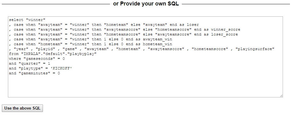
Enter the custom SQL in the “Provide your own SQL” and then hit the button “Use the above SQL”
Once the sql is submitted, InfoCaptor switches to the Visualizer tab and shows a nice compact list of dimensions and measures
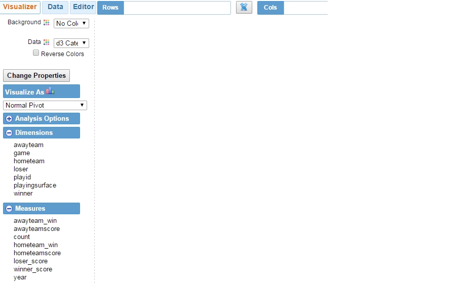
Befor we begin, we may want to enable the small checkbox just left of the refresh button. By default when you drag drop dimensions and measures in the row/col/values bucket InfoCaptor instantly runs the analysis. This is good for small datasets and RDBMS but since we are hitting the hadoop cluster it is often helpful to defer the refresh until we are done adjusting the columns. This provides an added inconvenience of clicking the refresh button but when you are working with Hive, imagine the relief of not having to wait 40 to 90 seconds of Hive map reduce jobs to finish and update the visualizations after every change.

Let us being our analysis
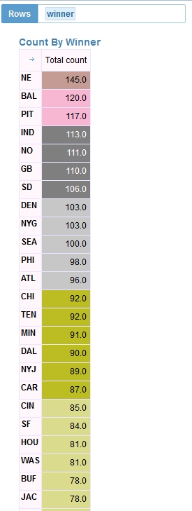
1. Who won the most NFL games?
2. Who won the most games against which losing team?
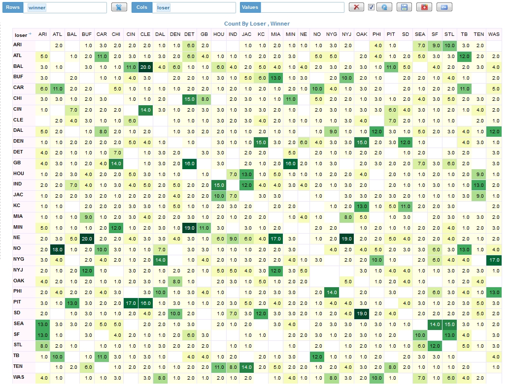
The winning team is the list going top to bottom on the left axis. The losing team is listed horizontally.
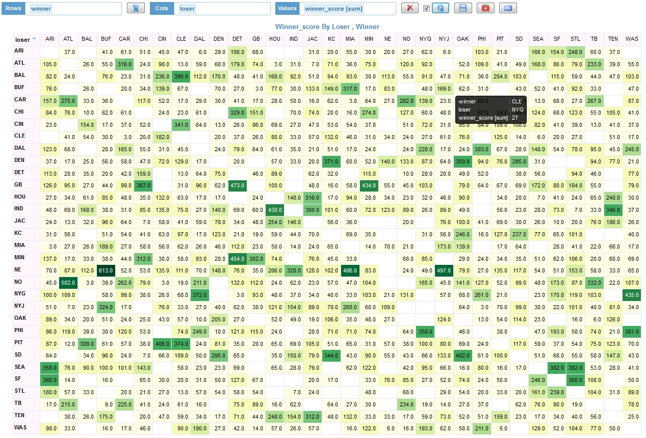
We can look at the same analysis by adding winning score
3. Is there a correlation between playing surface and the winning team?
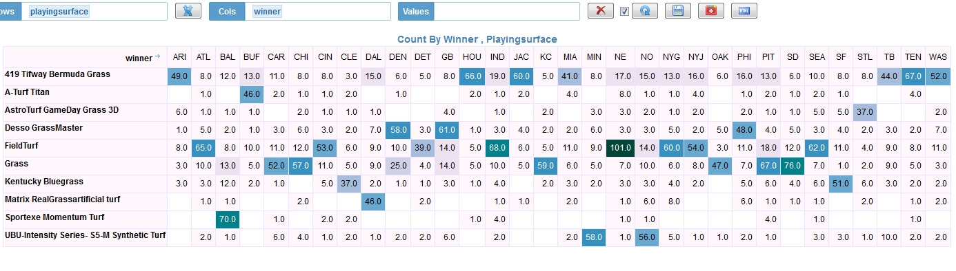
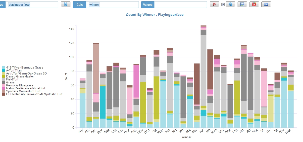
Looks like certain teams may have winning advantage on FieldTurf vs Tifway Bermuda Grass.
This was just an attempt to analyze the NFL dataset using Hadoop. Stay tuned for more.